Table of Contents
Study population
The study protocol was approved by the institutional review board (IRB) of Mississippi State University and all research was performed in accordance with the guidelines and regulations described in the IRB protocol. A total of 14 subjects with no history of CVDs and from diverse backgrounds were recruited (50% White, 21.5% Black, 21.5% Asian, and 7% mixed). Table 1 shows the study population’s age, height, weight, and body mass index (BMI). The subjects signed an informed consent form and completed a short survey about their health conditions prior to the study.
Experimental protocol
All subjects were instructed to lay supine on a bed without additional body movements (Fig. 1a). To minimize the respiration noise, data was acquired during a 15-s breath-hold at the end of inhalation followed by another 15-s breath-hold at the end of exhalation.

Experimental setup: (a) subjects were asked to lay down in a supine position. A smartphone was held by a phone holder to videotape the subject’s chest. (b) The arrangement of the signal and video acquisition systems.
Vision-based SCG (SCG\(\mathrm{^{v}}\))
A smartphone (iPhone 13 Pro, Apple Inc, Cupertino, CA) was used to videotape the upper chest of the subjects with an acquisition speed of 60 frames per second (fps) and resolution of \(3840 \times 2160\). A phone holder was used to keep the smartphone stationary with the back camera facing the subject’s chest. To minimize the phone vibrations, a Bluetooth remote control was used to start and stop the recording. We placed three texture-patterned QR codes on the chest surface as a high-contrast artificial region of interest to be tracked by our computer vision algorithm, since the sufficient intensity variation in the target region provides reliable recognition and matching in target tracking32.
Gold-standard SCG signals (SCG\(\mathrm{^{g}}\))
In order to validate the vision-based SCG signals, a triaxial accelerometer (356A32, PCB Piezotronics, Depew, NY) was placed underneath each QR code. The accelerometers were then attached to three locations on the sternum including the manubrium, the fourth costal notch, and the xiphoid process. A signal conditioner (482C, PCB Piezotronics, Depew, NY) was used to amplify the accelerometer outputs with a gain factor of 100. The amplified signals (i.e., SCG\(^\mathrm{{g}}\)) were then recorded using a data acquisition system, DAQ, (416, iWorx Systems, Inc., Dover, NH) with a sampling frequency of 5000 Hz.
The accelerometer outputs and the chest videos were recorded simultaneously using two independent systems (i.e., the DAQ and phone) with different sampling frequencies. Therefore, to synchronize the SCG\(^\mathrm{{g}}\) and SCG\(^\mathrm{{v}}\) signals in the later stages of the data analysis, a microphone was connected to both of these systems and was tapped at the beginning and end of each recording. These taps were then identified in the audio of the video and the sound signal recorded by the DAQ to synchronize the signals. In addition, ECG signals were recorded in each experiment (iWire-B3G, iWorx Systems, Inc., Dover, NH) and were used for SCG segmentation as will be described later. Figure 1b shows the sensor locations and the direction of x and y-axes in this study.
Vision-based SCG measurement method
Our vision-based SCG signal measurement is based on tracking artificial targets (i.e., QR codes) on the chest surface. As shown in Fig. 2, the videos were pre-processed after the video acquisition. We then employed a target-tracking algorithm to measure the displacement of the target regions. Camera calibration was then performed to convert the displacements from pixels to millimeters. Finally, we computed the acceleration signal from the displacements. Overall, the pipeline consists of four steps: (1) preprocessing; (2) vision-based tracking and displacement calculation; (3) camera calibration; and (4) acceleration calculation. Each step is described below.

Vision-based SCG estimation pipeline. The pipeline consists of four main steps: preprcessing, target tracking, camera calibration, and acceleration calculation.
Preprocessing
To calculate the SCG signals in the x and y directions as depicted in Fig. 1b, the videos were rotated, if needed, on a case-by-case basis such that the QR codes are aligned with the camera’s x- and y-axes. This step was done for each QR code separately to ensure that the x and y-axes of the video and accelerometers are as aligned as possible.
Vision-based tracking and displacement calculation
Computer vision methods are widely used for object tracking and displacement measurement in videos. Vision-based displacement estimation methods, such as tracking techniques and optical flow compute relative displacement by correlating successive image frames in a video. Template matching is the most prevalent tracking technique, which works by searching for the image regions that are most similar to a reference template. In the present study, we employed an optical flow-based template tracking method to extract the displacement information of the target regions on the chest. More specifically, we used the Lucas–Kanade template tracking algorithm33 to measure the displacement of the QR codes attached on the chest. In this regard, we adapted the unified approach proposed in34 for the Lucas–Kanade method for QR code tracking, with the goal of minimizing the sum of the squared error between two images, i.e., the QR code itself and a video frame in which the QR code is being searched for. The minimization is done based on warping the video frame onto the coordinate frame of the QR code. Since this optimization is nonlinear, it is performed iteratively solving for increments to update previously known warping parameters.
Given a chest video sequence I(x), let \(I_n({x})\) represents the \(n\)th video frame in which we looked for a region to match the QR code template, where \({x}=(x,y)^T\) is a column vector that contains the pixel coordinates and \(n=1,2,\dotsc ,N\) represents the frame number. Template QR(x) is the target region defined from the first frame \(I_1({x})\) of the chest video. The motion of the QR code was then calculated by mapping the QR(x) to the successive frames \(I_n({x})\). The mapping was done using a warp function W(x; u), which was parameterized by vector \({u}=(u_1,\dotsc ,u_k)^T\). The warp function W(x; u) transforms the pixel x in the coordinate frame of the QR(x) to the sub-pixel position W(x; u) in the coordinate frame of the video frame \(I_n({x})\). Assuming that the QR code is flat, parallel to the camera plane, and not rotated, the warp function W(x; u) can be then computed using the following 2D image transformation, where the parameters \({u}=(u_1,u_2)^T\) is the motion vector.
$$\begin{aligned} {{W(x;u)} = \left( \begin{array}{cc} x+u_1 \\ y+u_2 \end{array}\right) } \end{aligned}$$
(1)
The goal of the tracking algorithm is now to find optimal parameters u such that the warped image \(I_n({W(x;u)})\) and the QR(x) are perfectly aligned. The region that matches the QR code in a new frame is determined by optimizing the parameters u to minimize the sum of squared difference error between \(I_n({W(x;u)})\) and QR(x) as
$$\begin{aligned} {E=\sum _{{x}\in QR}\left[ I_n({W(x;u)})-QR({x})\right] ^2} \end{aligned}$$
(2)
where the error between the intensity of each pixel x of the QR code and its corresponding pixel in the video frame \(I_n({W(x;u)})\) is measured. In order to compute \(I_n({W(x;u)})\), it is necessary to interpolate the image \(I_n\) at the sub-pixel positions W(x; u). The minimization of the expression in (2) is a non-linear optimization problem, which is solved by iteratively updating the parameters u using the increments \({\Delta u}\) assuming that the current estimation of u is known. Consequently, (2) can be rewritten as
$$\begin{aligned} E=\sum _{{x}\in QR}\left[ I_n({W(x;u+\Delta u)})-QR({x})\right] ^2 \end{aligned}$$
(3)
and parameters u are iteratively updated as
$$\begin{aligned} {{u\leftarrow u+\Delta u}} \end{aligned}$$
(4)
The non-linear (3) can be linearized by employing the first-order Taylor approximation of \(I_n({W(x;u+\Delta u)})\) as
$$\begin{aligned} {I_n({W(x;u+\Delta u)}) = I_n({W(x;u)})+{\nabla I_n}\frac{\partial {W}}{\partial {u}}\Delta {u}} \end{aligned}$$
(5)
where \({\nabla I_n} = \left( {\partial I_n}/{\partial x}, {\partial I_n}/{\partial y} \right)\) represents the gradient of the video frame \(I_n\) evaluated at the current estimation of the warp W(x; u), and \({\partial {W}}/{\partial {u}}\) is the Jacobian of the warp function W(x; u). The first-order approximation of \(I_n({W(x;u+\Delta u)})\) from (5) can be substituted in (3) as
$$\begin{aligned} {E=\sum _{{x}\in QR}\left[ I_n({W(x;u)})+{\nabla I_n}\frac{\partial {W}}{\partial {u}}\Delta {u}-QR({x})\right] ^2} \end{aligned}$$
(6)
Minimization of the error function in (6) is a least-squares problem that can be solved by taking partial derivative of the error function E with respect to \({\Delta u}\) as
$$\begin{aligned} \frac{\partial E}{\partial {\Delta u}}=&2\sum _{{x}\in QR}\left[ {\nabla I_n}\frac{\partial {W}}{\partial {u}} \right] ^T [ I_n({W(x;u)}) +{\nabla I_n}\frac{\partial {W}}{\partial {u}}\Delta {u}-QR({x}) ] \end{aligned}$$
(7)
and then set \({\partial E}/{\partial {\Delta u}}=0\), which results in
$$\begin{aligned} {{\Delta u} = H^{-1}\sum _{{x}\in QR}\left[ {\nabla I_n}\frac{\partial {W}}{\partial {u}} \right] ^T\left[ QR({x})-I_n({W(x;u)}) \right] } \end{aligned}$$
(8)
where H represents the \(n\times n\) Hessian matrix from the Gauss–Newton approximation and is defined as
$$\begin{aligned} {H=\sum _{{x}\in QR}\left[ {\nabla I_n}\frac{\partial {W}}{\partial {u}} \right] ^T\left[ {\nabla I_n}\frac{\partial {W}}{\partial {u}} \right] } \end{aligned}$$
(9)
The steps in (8) and (4) are iterated until the convergence of u (i.e., \(\Vert {\Delta u}\Vert \le \epsilon\), where \(\epsilon\) is a threshold). We also defined a limit for the maximum number of iterations \(i^{max}\) to reduce the computational cost. The pseudo-code of our vision-based tracking is shown in Algorithm 1.

Camera calibration
To convert the displacement obtained by the target tracking algorithm from pixel to millimeter, a geometric relationship between the 2D image coordinate system and the world coordinate system needs to be established. This was done by the camera calibration process. When calibrating the camera, we attempted to align the camera coordinate system with the world coordinate system. The scaling factor is one of the most common ways to calibrate a camera for measuring displacement. When the optical axis of the camera is perpendicular to the object plane, all points on that plane can be assumed to have the same depth of field and can be similarly scaled down to the image plane. Generally, the scaling factor can be computed using the following two methods35. First, \(SF_1=D_{mm}/D_{pixel}\) computes the ratio of the physical dimension of the object surface in millimeters or inches in the world coordinate system to the corresponding dimension in pixels in the image frame, where \(D_{mm}\) is the physical length of the artificial target in millimeter, and \(D_{pixel}\) is the corresponding pixel length (Fig. 3a). Second, \(SF_2=d\times p/f\) is based on the ratio of the distance between the camera and the target object to the focal length of the camera. Here, d is the distance from the camera to the object surface, f is the focal length, and p is the unit length of the camera sensor (\(\mu\)m/pixel). In this study, since the image plane was parallel to the motion of the target region, we employed the \(SF_1\) scaling factor. For the unit conversion from image pixels to millimeters, we first measured the actual physical size of the QR code, and then calculated the pixel dimension of the same QR code on the image, as illustrated in Fig. 3b. Using these two values, we then determined the scaling factor.

Camera calibration and calculating the scaling factor. (a) Pinhole camera model, (b) schematic diagram of scaling factor calculation for converting the pixel unit to length unit (mm). \(D_{mm}\) and \(D_{pixel}\) are the physical distance of two points in millimeters and the distance of the same points in the image pixel, respectively.
Acceleration calculation
After calculating the displacement signal and converting it into millimeters, the acceleration signal (i.e., SCG\(^\mathrm{{v}}\)) was derived by calculating the second derivative of the displacement signal.
Validation of vision-based SCG estimations
We validated our computer vision pipeline by comparing the SCG estimations with the gold-standard signals in time and frequency domains.

Overview of the gold-standard SCG\(^\mathrm{{g}}\) and vision-based SCG\(^\mathrm{{v}}\) preprocessing. The output of the microphone was recorded simultaneously by both the camera and DAQ to synchronize the signals. The raw SCG\(^\mathrm{{g}}\) was bandpass filtered and the SCG\(^\mathrm{{v}}\) was resampled to 5000 Hz. Both signals were then segmented using the ECG R waves, and the ensemble averages of their segments were computed. The time domain similarity analysis was performed between the ensemble averages of the SCG segments. For the time–frequency analysis, the whole preprocessed signals were used.
Signal preprocessing
To compare the SCG signals recorded by the accelerometers with those estimated from the chest video, both SCG\(^\mathrm{{g}}\) and SCG\(^\mathrm{{v}}\) signals were first preprocessed. Figure 4 shows an overview of the signal processing pipeline in this study. The accelerometer outputs were filtered using a band-pass filter with cutoff frequencies of 1 and 30 Hz. This was done because the SCG estimations from the video could capture vibrations up to half of the camera acquisition speed (i.e., 60 fps). Additionally, the vision-based SCG signals were resampled using linear interpolation to 5000 Hz (i.e., the sampling frequency of the gold-standard signals). The raw SCG\(^\mathrm{{v}}\) with the sampling frequency of 60 Hz was missing some waveform features such as the curvature between two consecutive sample points. The resampling step was done to obtain a smoother SCG\(^\mathrm{{v}}\) by reconstructing the missed features and had a minimal effect on the signals’ contents in time and frequency domains. The resampling step also included the employment of an FIR antialiasing lowpass filter and accounted for the delay introduced by the filter. SCG signals were then segmented into cardiac cycles using the ECG R waves identified using Pan–Tompkin algorithm36,37. First, the average cardiac cycle duration in terms of the number of sample points, \(n_c\), was calculated for each subject using the ECG RR intervals. Then, SCG segments were defined as \(SCG(n_i-n_c/4:n_i+3 \times n_c/4)\), where \(n_i\) denotes the time index of the ith ECG R wave.
Time domain similarity
The ensemble averages of the SCG segments, \(\overline{\text {SCG}}^{g}\) and \(\overline{\text {SCG}}^{v}\), were calculated and used for the time domain similarity analysis. The ensemble averaging helped remove the beat-to-beat variability and noise. The Pearson correlation coefficient between \(\overline{\text {SCG}}^{g}\) and \(\overline{\text {SCG}}^{v}\) was calculated for the signals recorded from all three locations. This coefficient represents how closely the two signals are correlated. However, any time lags between two similar signals may lead to a low correlation coefficient. Therefore, in this study, we also used dynamic time warping (DTW) to assess the similarity of the signals38. For this purpose, Euclidean distances between the ensemble average of the vision-based and gold-standard SCG segments, \(D(\overline{SCG}\mathrm{^{g}},\overline{SCG}\mathrm{^{v}})\), were first calculated using DTW while the warping path was restricted to be within a 5% distance threshold from the straight-line fit. The similarity index, S, between the ensemble averages was then defined and calculated as
$$\begin{aligned} S_x(\overline{SCG}_x^g,\overline{SCG}_x^v) = \frac{M(\overline{SCG}_x^g) - D(\overline{SCG}_x^g,\overline{SCG}_x^v)}{M(\overline{SCG}_x^g)} \end{aligned}$$
(10a)
$$\begin{aligned} S_y(\overline{SCG}_y^g,\overline{SCG}_y^v) = \frac{M(\overline{SCG}_y^g) - D(\overline{SCG}_y^g,\overline{SCG}_y^v)}{M(\overline{SCG}_y^g)} \end{aligned}$$
(10b)
where \(M(\overline{SCG}\mathrm{^{g}})\) is the maximum of the absolute value of the gold-standard SCG\(^\mathrm{{g}}\) segments multiplied by the length of one segment, i.e., \(n_c\). This normalized similarity index is always in the range of \(\left[ 0,1 \right]\).
Wavelet coherence analysis
The correlation between the gold-standard and vision-based SCG signals in the time–frequency plane was calculated using magnitude-squared wavelet coherence (\(C_{g,v}\)) as39
$$\begin{aligned} C_{g,v}(a,b)=\frac{\left| \mathscr{S}(C_g^{*}(a,b) C_v(a,b)) \right| ^2}{ \mathscr{S}(\left| C_g(a,b) \right| ^2) . \mathscr{S}(\left| C_v(a,b) \right| ^2)} \end{aligned}$$
(11)
where \(C_g(a,b)\) and \(C_v(a,b)\) are the continuous wavelet transforms of the signals SCG\(^\mathrm{{g}}\) and SCG\(^\mathrm{{v}}\) at scales a and positions b. \(\mathscr{S}(\cdot )\) is a smoothing function in time and scale, and the superscript \(*\) is the complex conjugate operator. The coherence was calculated using the analytic Morlet wavelet since previous work showed that Morlet wavelet estimates the frequency content of SCG signals more accurately than other mother functions40. The correlations were calculated for the duration of the recordings and in the range of 0–30 Hz. \(C_{g,v}\) is always in the range of \(\left[ 0,1 \right]\), with \(C_{g,v}=1\) indicating the highest correlation between the two signals in the frequency domain.
Heart rate estimation
The heart rate (HR) of subjects was estimated using SCG\(^\mathrm{{v}}\). To evaluate the accuracy of these estimations, they were compared with the gold-standard HR values obtained from the ECG signals (\(HR_{ECG}\)). \(HR_{ECG}\) was calculated in beats per minute (bpm) by determining the temporal indices of the ECG R peaks using the Pan–Tompkin algorithm, and then substituting them in Eq. (12):
$$\begin{aligned} { HR_{ECG}^i = \frac{1}{t(n_{i+1})-t(n_i)} \times 60 } \end{aligned}$$
(12)
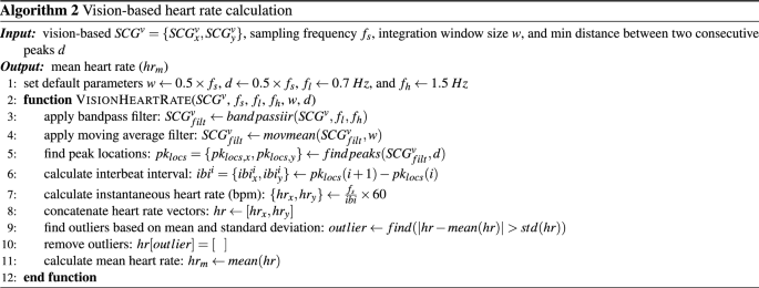
where, \(n_i\) represents the time index of the ith ECG R peak. To estimate the HR from SCG\(^\mathrm{{v}}\) (\(HR_{SCG}\)), we developed an algorithm based on bandpass filtering of the signals and finding the peaks of the filtered signals (Algorithm 2).